


 Global Sourcing Spotlight: Golf, Friedman, and the Benefits of Global Sourcing
 Nolan’s Notes: Coming to Terms With AI
 The Knowledge Base: A CM’s Perspective on Box Build Practices
Virtual Sample "Analyzing the Shipped Component"
December 31, 1969 |Estimated reading time: 7 minutes
This technology permits examination and reconstruction of features neglected or unfocused upon before the part was used in the field.
By Tom Adams and Lawrence W. Kessler
A new mode of acoustic micro-imaging has been developed that collects and stores complete acoustic data throughout the entire volume of a sample, such as an integrated circuit (IC) package. From only one scan sequence, acoustic data are stored in a matrix file from which any of more than 20,000 different acoustic micrographs can be constructed. After a sample has been scanned (in the new mode), it can be shipped, put into service or be subjected to other forms of testing. However, the sample's complete acoustic data will remain for later analysis.
Any feature within the sample can be imaged at any time even though the sample is not on hand, i.e., a "virtual sample" has been created. For example, the mode can enhance the detection of subtle material properties or bond-quality features.
Data Collection Basics: the C-SAM
In the acoustic-imaging process, an ultrasonic transducer scans the area of the sample, but at any given moment is positioned above a single X-Y point. Here, the transducer focuses a pulsed ultrasound beam into the sample. Later (microseconds or less), echoes from the various features along the beam within the sample return to the transducer where they are collected. The system that performs such imaging is the C-mode scanning acoustic microscope, or C-SAM.
Because the sample has a finite thickness, echoes from various depths (Z) arrive at the transducer at slightly different times, i.e., the pattern of echoes through the part from a single X-Y point on the surface has a time/depth dimension called the A-Scan. It is visible on an oscilloscope as a trace that shows echo waveforms at progressive depths within the sample. While the echo pattern is sharpest at the focus of the transducer, the area outside that region is distorted, with the image becoming progressively blurred.
In a typical application, a standard C-Mode image is produced in which an X-Y, 2-D display is constructed of the echoes from a selected depth. In this mode, only part of the A-Scan echo pattern is used (generally because only a single depth within the sample is of interest). The C-SAM system then selects only those echoes falling inside a time window (e.g., 1.2 to 1.25 µsec) corresponding to the depth of interest, the selection of which is called "gating."
The C-Mode image is made by applying the time window to all X-Y positions. This is referred to as a time-domain image (vs. frequency-domain images, described below). Then, at each X-Y position, only echo peak intensity value and polarity within the gate are displayed; information on other echoes is lost.
In the standard C-Mode, sample information is limited by the parameter restrictions of the original scan. Because the A-Mode is not saved, neither can the data be regated nor the echoes be reprocessed to create different image information. However, the standard C-Mode is very useful and has been the "norm" since the acoustic micro-imaging development.
 Figure 2. One benefit of using a data file is speed. Because no physical scanning of the sample is involved, moving the gate (green lines) instantly produces a new C-Mode image (top right). Making an FFT image (bottom right) by moving the red bar to the frequency of interest takes a few seconds.
null
Rescanning Without the Sample
The virtual sample is created in the new acoustic micro-imaging mode and can be rescanned at any depth with any gate and any focus position. The echoes can be processed digitally or frequency-filtered to bring out subtle bond qualities or material property information. Known as the virtual rescanning mode (VRM), the development is significant because it can record entire A-Mode patterns for all volumetric elements (voxels) of a sample (Figure 1).
In the VRM mode, the C-SAM quickly scans the actual sample at increasing depths. However, instead of collecting only the peak value of a single echo, it collects the actual echo waveforms of all the echoes at each X-Y location. Thus, from all focused segments of A-Scan data at each depth, a master A-Scan is created for each X-Y position for preservation as the matrix file. Collectively, these data constitute the virtual sample, which can be rescanned in an infinite number of ways. The mode can, with some justification, be referred to as a 4-D technique because the matrix file contains X, Y and Z as well as time data.
Early field experience shows that the matrix file can be extremely useful. For example, with a field failure of an IC package, engineers can use the virtual sample acoustic file for comparison studies. It also can be used to interpret changes in a package after thermal stress testing, even if a defined defect has not yet occurred.
 Figure 3. At top left (a) is the rescanned C-Mode image of one portion of a flip chip, which contains all ultrasonic frequencies reflected from the gated depth. The rest, (b) through (f), are FFT-filtered images containing only echoes ranging from 141 to 226 MHz. Contrast varies from frequency to frequency, and metallization on the chip appears variously dark and light; however, FFT-filteredimages display better contrast (and resolution) for such details.
null

null

null

null

null

null
Frequency-domain Imaging
Acoustic micro-imaging transducers range from 10 to 300 MHz and above. In conventional acoustic imaging, transducer choice determines spatial resolution, penetration and other parameters. Thus, if a sample is scanned with a 50 MHz transducer, one cannot manipulate the image data to produce a 10 or 100 MHz image. This is because the acoustic pulses themselves do not have sufficiently wide frequency content. However, the data file created by the VRM makes such manipulation possible, within limits. Data collected at 50 MHz can be used to create images showing the sample at frequencies from 30 to 70 MHz, and data collected at 300 MHz can be used to create images showing the sample at frequencies from 225 to 375 MHz. However, large excursions in frequency — e.g., those using a data file collected at 10 MHz to create 300 MHz C-Mode images — are not possible. The same sample can, of course, be scanned physically with various transducers.
Because the new mode collects all waveforms from all regions of the sample, it also can accommodate the frequency changes that may occur during reflection. For example, a pulse of 15 MHz ultrasound launched toward a material interface (e.g., molding compound to die face) may be reflected with a different frequency content than pulsed originally. This change — not otherwise detectable — may be indicative of the interface condition. The echo waveforms can be filtered by a fast Fourier transform (FFT), also called a frequency-domain algorithm, to isolate a given frequency (Figure 2). An FFT decomposes the waveform into sinusoids of different frequencies and identifies the different frequency sinusoids and their respective amplitudes. Frequency-domain imaging is valuable because specific features may yield more information at one frequency over another. The FFT filtering brings out image detail that may not be seen with conventional time-domain imaging.
Producing Images from the Data File
Images produced from the time-domain VRM mode do not necessarily look different from conventional C-mode images except that accuracy and resolution are maximized for images from any depth. The chief advantage over standard imaging is the ability to create any image from any other depth, including 2- and 3-D images. Achieving the same volume of data by conventional imaging would be impossible.
Figure 3 (on page 36) shows the reconstructed C-SAM image of a portion of a flip chip package together with FFT-filtered images at 141, 167, 175, 195 and 226 MHz. Bright solder bumps in the C-Mode image are defective probably because of cracks in the passivation layer rather than solder joint disbonding or cracking.
Each of the FFT-filtered images shows the virtual sample as it is imaged by echoes at a given frequency. One advantage to this type of imaging is that different acoustic frequencies are sensitive to different features within the sample. Overall, the lines of metallization on the chip are defined more sharply in the FFT-filtered images than in the multi-frequency C-Mode image. There are differences in contrast to the FFT-filtered images: the solder bump defects are bright in some, dark in others. Finally, it appears that the higher frequencies within the spectrum of frequencies from the sample are reflected from a slightly deeper level. Thus, in Figure 3, image 3f, at 226 MHz, actually is imaging at a level slightly deeper than that of image 3b at 141 MHz.
Conclusion
The newly developed VRM changes the nature of acoustic micro-imaging by broadening its ability to collect, analyze and display data. Previously developed modes have provided numerous methods for displaying acoustic data from specific regions of a sample in two or three dimensions. The new mode, however, permits data collection from all regions of the sample and displays such data with greater flexibility.
Tom Adams and Lawrence W. Kessler may be contacted at Sonoscan Inc., 2149 E. Pratt Blvd., Elk Grove Village, IL 60007; (847) 437-6400; Fax: 847 437-1550; E-mail: info@sonoscan.com.
Share on:


